In the opening episode, we explained what the Edge Ratio is and outlined the basic methodology for using it to develop strategies in StrategyQuant X. The sequel to this article is yet to come, which will be preceded by several analyses, in which we will try to understand the Edge Ratio to use it properly in strategy development.
Firstly let’s repeat what Edge Ratio is:
- Record MAE in pips and MFE in pips for each trade
- Divide each of them by ATR(14) to adjust for volatility and normalize for future Intermarket analysis
- Sum each value ( Normalized MAE and normalized MFE ) and divide with the total number of trades
- Edge ratio is the average volatility normalized MFE divided by average volatility normalized MAE
So the higher the MFE and simultaneously lower the MAE leads to the higher Edge Ratio. It means that the signal has a higher edge. ( The trade profit potential is higher than the loss potential ).
The objective of the analysis
Today’s analysis aims to find the relationship between Net Profit and Edge Ratio in the periods of True out-of-sample – 12, 26, 32 months and Edge Ratio in the building phase.
We will try to find whether higher Edge Ratio strategies during the measured building phase lead to positive results in true out-of-sample periods.
Data collection
How we will generate strategies/signals
For our analysis, we will create a template with the following structure: Strategy will be always in the market. It will enter a long trade whenever a long signal occurs. It will enter a short trade whenever a signal opposite to the long trade occurs.
We will thus observe the characteristics of the strategies generated based on this template
- Edge Ratio during the building phase
- Net Profit in True Out-of-sample period
- Edge Ratio in True Out-of-sample period
Sample size
For each instrument and time frame, we will draw a random sample of 10,000 strategies (a total of 30,000 strategies per instrument). To avoid a biased distribution of results, we will not use the genetic searching algorithms during mining strategies in the builder.
Markets
We will analyze EURUSD and GBPPY as well as futures on ES ( Mini SP500 ), XK ( Mini Soybean ), QO ( Mini Gold ), and CL ( WTI OIL ). For both currency pairs, we will use Darwinex’s normal fee structure. We will use a slippage of 0.5 pip. For the futures, we will use a slippage of 1 tick and a commission according to the futures price list AMP.
Builder settings
For currency pairs, we will use data from 1987-31.12.2017 ( in-sample + out-of-sample period)
For the futures contracts, we will use data from 2009-31.12.2 2017 ( In-sample + Out-of-sample period)
- 12 months True out-of-sample will be the period from 1.1.2018-31.12.2018
- 24 months True out-of-sample will be the period from 1.1.2018-31.12.2019
- 32 months True out-of-sample will be the period from 1.1.2018-31.12.2020
For statistical significance, we will only analyze strategies with an average of 25 signals per year.
We will use a total of 603 conditions in the builder. Part of them is the default part of StrategyQuant X, part of them is made by me using custom blocks.
HOW to use custom blocks: https://strategyquant.com/doc/strategyquant/custom-blocks/
What we are going to measure
- The correlations between the EDGE ratio in the building phase and between the Net Profit and Edge Ratio in out-of-sample
- Relative frequencies Edge Ratio in the building phase vs. the median values in the out-of-sample.
- Frequencies of Intervalised Edge Ratio in building phase by deciles vs. median Net Profit / Edge Ratio values in out-of-sample.
For the sake of brevity, in this blog post, we show the analysis of 60 Minute Time Frame EURUSD and futures contract ES ( E-mini SP500 ). In the appendix, you will find analytical tables on other markets and time frames.
Analysis
EUR USD 60 Minutes Time frame
Correlations ( Pearson ) between the key indicators
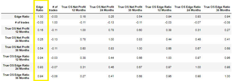
In the figure above, we see that the Pearson correlations between Edge Ratio in the building phase and Edge Ratio / Net Profit in the true out-of-sample periods are low. In other words, a higher Edge Ratio in the building phase does not imply a higher net profit in out-of-sample periods 12/24/32 months.
What is a good sign, however, is the high correlations between the Edge Ratio in the building phase and between the true out-of-sample periods of 12/24/32 months. So we can expect the potential of signals in the true out-of-sample period remains high.
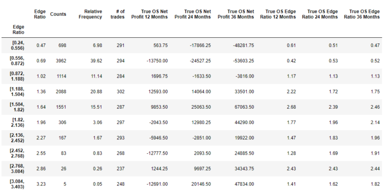
Binned Edge Ratio into 10 intervals
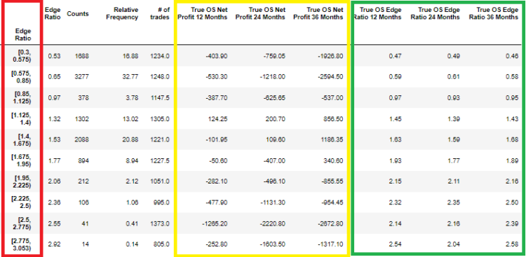
In the chart above, we have sorted the strategies by their Edge Ratio in the Building phase ( red frame ). In the yellow and green frames, we see the median values of true out-of-sample Net Profit and true out-of-sample Edge Ratio.
In the third column, we see the number of strategies – 1688 in the given interval. In the yellow frame, columns 6 to 8, we see the median value of Net Profit in out-of-sample periods of all strategies with Edge Ratio in the interval 0.3-0.575. In rows 10 to 12, we see the Edge Ratio in true out-of-sample.
Note, that despite the negative Net Profit Results in true out-of-sample, the Edge Ratio in true out-of-sample remains high.
Edge Ratio in equal-sized buckets based on deciles
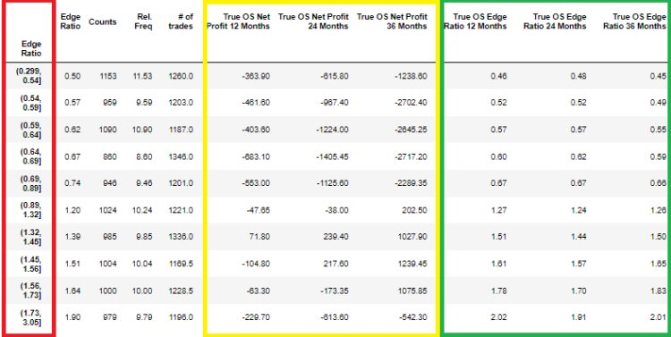
In the figure above we see Edge Ratio intervalized in deciles. In each interval, there is approximately the same number of strategies. A similar situation repeats itself. The out-of-sample true Net Profit results are inconsistent, while the out-of-sample true Net Profit and Edge Ratio remains consistently high.
ES – E-mini S&P 500 – 60 Minutes Time frame
Correlations ( Pearson ) between the key indicators.
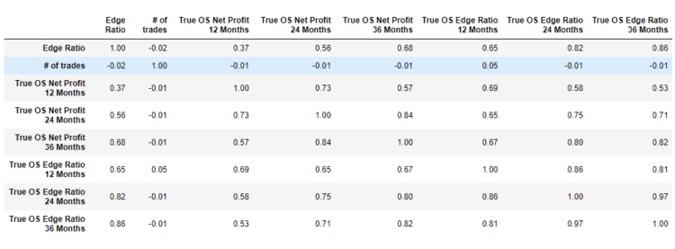
In the graph above, we see fairly strong correlations between Edge Ratio in the building phase and between Edge Ratio in the true-out-of-sample periods. The correlations between Edge Ratio and Net Profit true out-of-sample are also not insignificant. In other words, a higher Edge Ratio in the Build phase also leads to a higher Net Profit true out-of-sample periods.
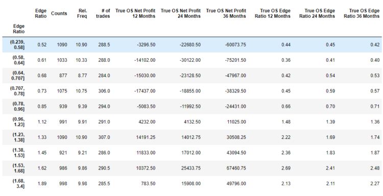
Binned Edge Ratio into 10 intervals
Using the frequency table, we can already see that higher values of Edge Ratio in the building phase don’t lead only to higher median values of true out-of-sample Edge Ratio, but also higher median values in the out-of-sample Net Profit. We can see the picture suggested by the correlation table in the example above.
Edge Ratio in equal-sized buckets based on deciles
In the picture above, we see the Edge Ratio in the building phase sorted in deciles. It means that there is roughly the same number of strategies in each interval. We see a similar picture. A higher edge ratio in the build phase leads to a higher Net Profit in the true-out-of-sample and Edge Ratio in the true-out-of-sample.
We can analyze all other instruments like EURUSD and ES similarly. For the sake of clarity, I am attaching the analysis tables in the appendix of this blog post. For each instrument, we need to follow the analysis procedure exactly as for EURUSD and ES.
You can find other datasets in this link
Conclusions
- The true out-of-sample Net Profit correlates with Edge Ratio in Building Phase very inconsistently
- Edge Ratio in Building Phase correlates with Edge Ratio in true out-of-sample. I.e. potential of trades remains also in true out-of-sample
- The problem lies in managing positions and exits from them.
- Methods of exiting positions need to be investigated.


 Tomas Vanek

Great article, but, unlike the “opening episode,” this article is unclear and difficult to follow. Typographical errors only make it worse. (Ration => Ratio, Decils => Deciles, Bined => Binned)
May be, it is better to explore correlation with Percentage Return, instead of Net Profit?
I am curious how Corr(ER, PctReturn) changes from In-Sample to Out-of-sample.
Hi Murty. The typos are fixed, thank you, I will implement your ideas in the next part.